Wednesday, September 29th Links

Today's exploration

Power Rule Practice on ThatQuiz.org

Unit 2 Assignment #1

Unit 2 Assignment #1 solutions

Derivatives

Today we started unit two: Derivatives.

Verbal: The derivative of a function at a point is the "instantaneous" rate of change of the function at that point. It is the slope of the tangent line at the point on the function's graph. In physics, the derivative finds the velocity at a moment in time.
Ex.) rise/run, displacement/time, bytes/sec, words/min...

Numeric: We used#4 from the test:

We used difference quotients to find approximate values. The difference quotient is obtained by subtracting the twoY1

values and dividing by the two X values. Using (X,Y1) values on each side of one gives the symmetric difference quotient.

To use nDeriv, the syntax is nDeriv(e^(X),X,1)
We found out that nDeriv is actually finding the symmetric difference quotient to give us the value. It is not, as Mr. O'Brien said, a "magical elephant" performing calculations.

Graphic:
We used #5 from the test:

We graphed with GeoGebra, adding in values (1, f(1)) and (4, f(4)). Connecting this lines gave us a secant line.

The slope shown above is the average rate of change: 2.28

The graph above shows the secant line in purple, and the tangent line in green. As we move the second point on the secant line closer to the first point, the slope of the secant line approaches the slope of the tangent line.

Algebraic:

This is the limit of the slope of the secant line as the second point approaches the point of tangency.

So, as an example:

We then did an example with 16c on our test. WolframAlpha confirms that the derivative of g(x)=1/x is 1/4. WolframAlpha can also find it using nDeriv.

A second form of the derivative definition:

Explained by the scanned graph (click for a larger image):

The "trick":

Links: A PDF showing an example of a derivative found algebraically can be found here. A good walkthrough of the whole idea is here.

Homework for next class is to finish Supercorrections. We will have Tuesday in class to work on them.

Marnie is the scribe for next class.

September 21, 2010. Limits, Continuity, and Derivatives Oh My!

We started class with a warm up, which was really just more practice with continuity. It really reinforced the two things we need to remember: what makes a function continuous or discontinuous. To recap, the three rules of continuity are: f(x) is continuous at point c if:

1) f(c) exists (not a hole or an asymptote, volcanic or otherwise)

2) limit of f(x) approaches c exists (no breaks or normal asymptotes)

3) the above limit is equal to f(c)

A function is continuous if it is continuous along all points within its domain.

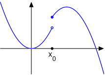
Also, remember the two types of discontinuity:

1) A removable discontinuity is a single point, either a hole or a single discontinuous value (in a piecewise defined function it would be a clause that said f(x) = 6 if x=6.)

2) A non-removable discontinuity is a jump, or break in an otherwise continuous graph

(see graph below)

This WILL be on the test Thursday, so study up.

After finishing with the warm up, we went over the quiz, which seemed to go reasonably smoothly for everyone. The only issues that came up were addressed quickly, though discontinuities did come up at least once.

From the quiz we jumped right into assignment 7 (remember that one, two posts down?). Specifically, we demonstrated how you could use different methods to solve the problems from 5, most importantly part c (with natural log of x in the numerator). We also covered number 8, and went over several methods to solve it. For average rate of change, we can just graph it, and draw a line between the two points. The slope of this line (called a secant line) is equal to the rate of change between those two points.

For the instantaneous rate of change, it gets kinda tricky. Firstly, knowing that instantaneous rate of change is also the derivative, we can use nDeriv on our calculators (nDeriv lives under the Math key, option #8). Secondly, we can plug it into wolframalpha and get a perfect answer. Finally, we can take

Using c as whatever point you are trying to find the instantaneous rate of change at, then solving the limit as we have been doing for ages now. This is a big idea, but WILL NOT be on the test Thursday.

Mr. O'Brien then handed out the next assignment (down below). It looks like a practice test (which it basically is) but it will be collected on friday along with #5,6,7. Use it however you like, but it might be a really big help on thursday's test.

Thursday's test will cover Limits and Continuity.

For study help we return to ucdavis, as well as voyaging into the realm of the complicated with Paul . Remember: Test Thursday, Study hard!

Class Link and Assignment #8

Warm up

Assignment #8

Assignment #8 solutions

Assignment #7

Assignment #7

Solutions

September 15, 2010: Continuity and Local Linearity

UPDATE (10/29/10): Here's another link called Local Linearity: Seeing is Believing. Check it out!

Here is a PDF version of the notes: link.
Sometimes, it takes the simplest explanations in order to understand the concept, so here's a link to Calculus for Dummies: Using Limits to Determine Continuity
and here's a link to a applet where you can visualize different functions and determine continuity

College searching sites

I came upon this blog post this morning and thought some of you might find it interesting:

http://www.freetech4teachers.com/2010/09/7-sites-to-help-students-choose-and.html

It reviews 7 sites to help students with their college search.

September 13, 2010 Scribe Post

We began class today by performing a warm up exercise concerning the indeterminate form. First we were to find f(x) and g(x) such that f(c)=g(c)=0 and is:
1.
a) 0
b) 17
c)
d) D.N.E.

In other words, you are looking for an indeterminate case where you get zero in the numerator and zero in the denominator, such that it has the following properties: the limit is 0 or 17 or or D.N.E., and the functions values are each zero when we evaluate at this thing that we are approaching. This is other wise known as the indeterminate form.

Then we were to attempt to find the following equations without technology:
2.
a)
b)
c)

Before the class revealed their answers, Mr. O'Brien commented on a key idea which is that a function doesn't have a limit in general, it has a limit at a point. So you are never going to just a and a function, you going to have x approaching something otherwise you cannot possibly have a value for the limit.

Next, in order to test our answers we checked to make sure we had a fraction limit and also that both the numerator and the denominator were zeros. And in order to find the limit values, we used a table to evaluate our functions.

By looking at the table we declared that an answer to a) for the first question is . This function has a limit which is approaching zero. This is because as x gets very close to zero, the y value gets closer and closer to zero as well.


Next, in order to find an answer to b) for the first question, we decided to look at the problem algebraically. We created the function which when evaluated equals 17. We then multiplied this by the fufoo (funny form of one) and it gave us . Both of the functions and are identical at all values except for 3 (because the fufoo caused a hole at 3). Mr. O'Brien also comments that there are an infinite amount of answers to this problem but the key is using the fufoo.

In order to find where the limit D.N.E., instead of creating a hole, we need to create a gap, a break, or a non removable discontinuity. And in order to get that we need to include absolute value on the numerator so the equation looks like this: . This means that as we approach zero from the left and the right we are not getting one value but two which means that the limit does not exist. In order to better visualize this I replicated the graph:

Overall for all three problems Mr. O'Brien emphasized that if you have any function you can add a hole to it and it does not change the limit value.

Lastly for c) we got . We had instead of because, when you reduce you get which gives you a volcano asymptote. This means that you will have an infinite value for y when you approach 0.


Next we evaluated the infinite limits for question 2 without a calculator. The first one is a natural log function which means the domain is everything above zero, there is no y intercept, and the x intercept is 1. Now to evaluate we look at t as it approaches infinity which is zero. This means that we are considering the natural log of zero which is negative infinity. Because as x approaches zero it has a vertical asymptote. So if you know the parent function you can reason through the limit without the technology.

Now for b) and c) of question 2 it helps to think about how fast the fractions are growing. For b) the limit is approaching zero because the numerator is approaching infinity slower than the denominator. For c) the numerator is growing so much faster than the denominator making the limit be infinity.

Next we evaluated the quiz. An important not was that for number 4 you need to include the actual value which is opposed to 1.732 which is an approximate value. In addition, Mr. O'Brien noted that by the end of class, the entire first side of the quiz should be able to be done without a calculator. For number 7 Mr. O'Brien noted that students need to provide an explanation or a counter example.
Next we "NAG" (to take a look at the numeric, algebric, graphic) the function . We determined that the limit was 1 and there was a gap at (0,1). The graph looked like this:

Mr. O'Brien then adds that you cannot see the hole, but you know that there is a hole because the function is not defined at zero. Next we looked at this algebraically because this one limit is the foundation of all of the calculus of trigonometry that we are going to do. We noticed that as x gets bigger and bigger the end behavior get smaller and smaller giving you a horizontal asymptote of zero. This is because the denominator gets bigger and bigger and the numerator is oscillating between 1 and negative 1.


We now turned our attention to The Squeeze Theorem (aka The Sandwich Theorem) which states: If on some open interval containing c and then .

We then reviewed an example of this which is and looks like this:

This has to do with the squeeze theorem because. This concept is better viewed in the graph:
Here we can see a visual of the squeeze therom. We know that the limit of both and is zero meaning that the limit of is zero as well.

Next in order to look at as a sandwich equation we looked at the following diagram:

In the diagram: AD= and BC=
Now by using and we were able to come up with the following equation:

then multiplied by 2 and got:
then we divided by and got:
Lastly, we reciprocated the following equation and got:

Now since and we have applied the sandwich theorem for .

An additional diagram that might be helpful is the one Lange used in her blog:

In the last two minutes of class we were not able to complete two example problems which would help further our understanding of this theorem. So, it would be helpful to review example 3 and 4 on page 87-88 tonight before the homework. In addition, the following website http://www.math.ucdavis.edu/~kouba/CalcOneDIRECTORY/squeezedirectory/SqueezePrinciple.html provides numerous examples of the Squeeze theorem which will help as well.